
The Exposure Calculator answers the oldest question in astrophotography – how long should my subs be? – with a full camera-and-sky noise model instead of folklore. It has two modes: SNR Efficiency for deep-sky work, and Exoplanet Star for point-source photometry where saturation control is everything.
Equipment & Camera Model #
Pick a telescope and camera from your Equipment library; the calculator pulls focal length, aperture, and reducer from the scope and pixel size, read noise, full well, and QE from the camera, displaying the derived image scale (206.265 × pixel size / focal length). If your camera has defined gain modes, choose one and the read noise / full well / gain fields update to that mode’s values – all three are overridable for what-if analysis.
Sky, Target & Exposure Inputs #
- Bortle Class (1-9) and SQM – linked in both directions; the sky flux in the model comes from the SQM value, your aperture, pixel scale, and QE.
- FWHM (arcsec) – seeing; spreads target light over more or fewer pixels.
- Target Type – twelve presets with realistic surface-brightness flux values, from Bright Emission Nebula (2.0 e-/px/s) down to IFN / Galactic Cirrus (0.02), plus Custom for your own value.
- Filter – twelve options from Luminance through 3nm narrowband to dual-band and IR, each carrying measured sky- and signal-transmission factors (a 3nm Ha filter passes ~1% of skyglow – this is why narrowband laughs at light pollution).
- Sub length, binning (1×1-4×4), bias, sensor temperature, dark current – the housekeeping terms; dark current follows the doubling-per-6°C rule from your entered temperature.
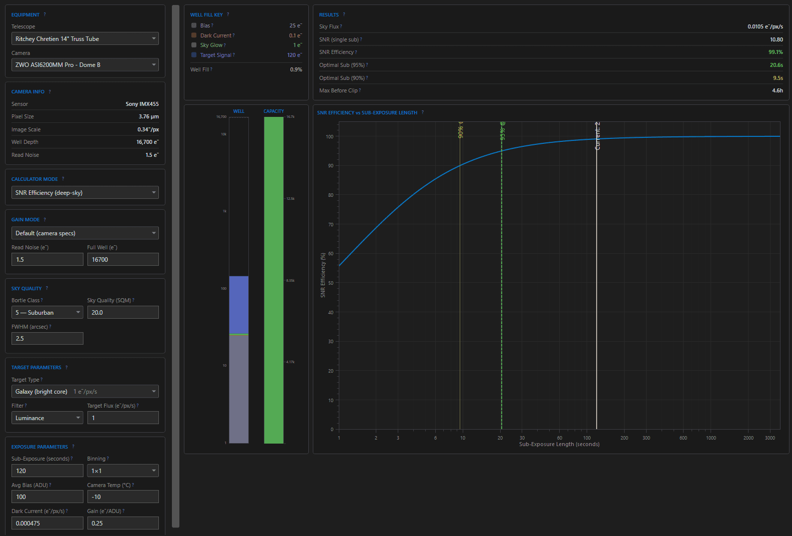
SNR Efficiency Mode: the Results #
The model computes single-sub SNR, then expresses it as efficiency – your SNR versus a hypothetical read-noise-free camera. That framing makes the answer actionable:
| Result | Meaning |
|---|---|
| SNR (single sub) | signal × t / √(total noise) for one frame |
| SNR Efficiency % | how close you are to ideal – green ≥90%, yellow 70-90%, red <70% |
| Optimal Sub (95%) | exposure where read noise costs you only 5% – the sweet spot |
| Optimal Sub (90%) | the practical minimum worth using |
| Max Before Clip | where the brightest pixel hits full well |
The key insight the chart makes visceral: past the 95% point, longer subs gain almost nothing while costing you more ruined frames per guiding hiccup or cloud. The curve plots efficiency against sub length (1-3600s) with your current sub marked, so you can see exactly where you sit.
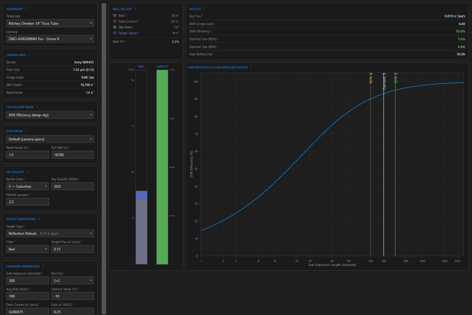
The Well-Fill Visualization #
The stacked bar shows where your electrons actually come from at the current settings – bias, dark, sky, and signal stacked on a log scale up to full well. One glance tells the story of your site: under Bortle 8 skies with a luminance filter, the sky bar dwarfs the signal bar – and the calculator is quietly explaining why sub length barely matters there and why the narrowband filters transform the picture.
Exoplanet Star Mode #
Transit photometry inverts the problem: one bright star, and the goal is keeping its peak pixel at a healthy well fraction (50% is the classic sweet spot) – saturated means ruined, too shallow wastes precision. Inputs: star V-magnitude, target well %, optical throughput, airmass and extinction, and spectral type (O through M) – the star’s color changes how its V magnitude translates into your imaging band.
Results: the Recommended Exposure headline, star flux and in-band magnitude, peak pixel rate, per-frame aperture SNR and photometric precision in millimagnitudes (a typical transit is 5-20 mmag deep – the number tells you if you can see it), and the system zeropoint.